System of linear equations of the 3rd order. Solving systems of linear algebraic equations, solution methods, examples. V.S. Shchipachev, Higher Mathematics, ch.10, p.2
Consider a system of 3 equations with three unknowns
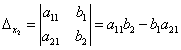
Using third-order determinants, the solution of such a system can be written in the same form as for a system of two equations, i.e.
 (2.4)
(2.4)
if 0. Here
It is Cramer's rule solving a system of three linear equations in three unknowns.
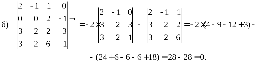
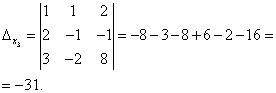
Example 2.3. Solve a system of linear equations using Cramer's rule:

Solution . Finding the determinant of the main matrix of the system

Since 0, then to find a solution to the system, you can apply Cramer's rule, but first calculate three more determinants:

Examination:

Therefore, the solution is found correctly.
Cramer's rules obtained for linear systems of the 2nd and 3rd order suggest that the same rules can be formulated for linear systems of any order. Really takes place
Cramer's theorem. Quadratic system of linear equations with a non-zero determinant of the main matrix of the system (0) has one and only one solution, and this solution is calculated by the formulas
 (2.5)
(2.5)
where – main matrix determinant, i – matrix determinant, derived from the main, replacementith column free members column.
Note that if =0, then Cramer's rule is not applicable. This means that the system either has no solutions at all, or has infinitely many solutions.
Having formulated Cramer's theorem, the question naturally arises of calculating higher-order determinants.
2.4. nth order determinants
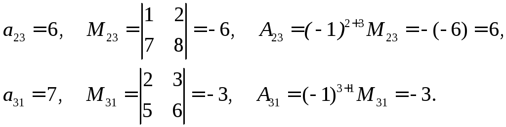
Additional minor M ij element a ij is called the determinant obtained from the given by deleting i-th line and j-th column. Algebraic addition A ij element a ij is called the minor of this element, taken with the sign (–1) i + j, i.e. A ij = (–1) i + j M ij .
For example, let's find minors and algebraic complements of elements a 23 and a 31 determinants

We get
Using the concept of algebraic complement, we can formulate the determinant expansion theoremn-th order by row or column.
Theorem 2.1. Matrix determinantAis equal to the sum of the products of all elements of some row (or column) and their algebraic complements:
 (2.6)
(2.6)
This theorem underlies one of the main methods for calculating determinants, the so-called. order reduction method. As a result of the expansion of the determinant n th order in any row or column, we get n determinants ( n–1)-th order. In order to have fewer such determinants, it is advisable to choose the row or column that has the most zeros. In practice, the expansion formula for the determinant is usually written as:

those. algebraic additions are written explicitly in terms of minors.
Examples 2.4. Calculate the determinants by first expanding them in any row or column. Usually in such cases, choose the column or row that has the most zeros. The selected row or column will be marked with an arrow.

2.5. Basic properties of determinants
Expanding the determinant in any row or column, we get n determinants ( n–1)-th order. Then each of these determinants ( n–1)-th order can also be decomposed into a sum of determinants ( n–2)th order. Continuing this process, one can reach the determinants of the 1st order, i.e. to the elements of the matrix whose determinant is being calculated. So, to calculate the 2nd order determinants, you will have to calculate the sum of two terms, for the 3rd order determinants - the sum of 6 terms, for the 4th order determinants - 24 terms. The number of terms will increase sharply as the order of the determinant increases. This means that the calculation of determinants of very high orders becomes a rather laborious task, beyond the power of even a computer. However, determinants can be calculated in another way, using the properties of determinants.
Property 1 . The determinant will not change if rows and columns are swapped in it, i.e. when transposing a matrix:
 .
.
This property indicates the equality of rows and columns of the determinant. In other words, any statement about the columns of a determinant is true for its rows, and vice versa.
Property 2 . The determinant changes sign when two rows (columns) are interchanged.
Consequence . If the determinant has two identical rows (columns), then it is equal to zero.
Property 3 . The common factor of all elements in any row (column) can be taken out of the sign of the determinant.
For example,

Consequence . If all elements of some row (column) of the determinant are equal to zero, then the determinant itself is equal to zero.
Property 4 . The determinant will not change if the elements of one row (column) are added to the elements of another row (column) multiplied by some number.
For example,

Property 5 . The determinant of the matrix product is equal to the product of the matrix determinants:
Practical work
"Solution of systems of linear equations of the third order by Cramer's method"
Goals of the work:
expand the understanding of the methods for solving the SLE and work out the algorithm for solving the SLE by the Cramor method;
to develop the logical thinking of students, the ability to find a rational solution to the problem;
to educate students in the accuracy and culture of written mathematical speech when they make their decision.
Basic theoretical material.
Cramer's method. Application for systems of linear equations.
A system of N linear algebraic equations (SLAE) with unknowns is given, the coefficients of which are the elements of the matrix , and the free members are the numbers
The first index next to the coefficients indicates in which equation the coefficient is located, and the second - at which of the unknowns it is located. 
If the matrix determinant is not equal to zero
then the system of linear algebraic equations has a unique solution. The solution of a system of linear algebraic equations is such an ordered set of numbers , which at turns each of the equations of the system into a correct equality. If the right sides of all equations of the system are equal to zero, then the system of equations is called homogeneous. In the case when some of them are nonzero, non-uniform ![]() If a system of linear algebraic equations has at least one solution, then it is called compatible, otherwise it is incompatible. If the solution of the system is unique, then the system of linear equations is called definite. In the case when the solution of the compatible system is not unique, the system of equations is called indefinite. Two systems of linear equations are called equivalent (or equivalent) if all solutions of one system are solutions of the second, and vice versa. Equivalent (or equivalent) systems are obtained using equivalent transformations.
If a system of linear algebraic equations has at least one solution, then it is called compatible, otherwise it is incompatible. If the solution of the system is unique, then the system of linear equations is called definite. In the case when the solution of the compatible system is not unique, the system of equations is called indefinite. Two systems of linear equations are called equivalent (or equivalent) if all solutions of one system are solutions of the second, and vice versa. Equivalent (or equivalent) systems are obtained using equivalent transformations. 
Equivalent transformations of SLAE
1) rearrangement of equations;
2) multiplication (or division) of equations by a non-zero number;
3) adding to some equation another equation, multiplied by an arbitrary non-zero number.
The solution of SLAE can be found in different ways, for example, by Cramer's formulas (Cramer's method)
Cramer's theorem. If the determinant of a system of linear algebraic equations with unknowns is nonzero, then this system has a unique solution, which is found by the Cramer formulas: ![]()
![]() - determinants formed with the replacement of the -th column, a column of free terms.
- determinants formed with the replacement of the -th column, a column of free terms.
If , and at least one of is nonzero, then SLAE has no solutions. If ![]() , then the SLAE has many solutions.
, then the SLAE has many solutions.
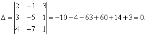
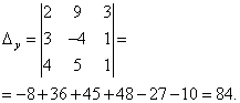
A system of three linear equations with three unknowns is given. Solve the system by Cramer's method
Solution. 
Find the determinant of the matrix of coefficients for unknowns

Since , then the given system of equations is consistent and has a unique solution. Let's calculate the determinants:


Using Cramer's formulas, we find the unknowns
So ![]() the only solution to the system.
the only solution to the system.
A system of four linear algebraic equations is given. Solve the system by Cramer's method.

Let us find the determinant of the matrix of coefficients for the unknowns. To do this, we expand it by the first line.


Find the components of the determinant:


Substitute the found values into the determinant
The determinant, therefore, the system of equations is consistent and has a unique solution. We calculate the determinants using Cramer's formulas:
Evaluation criteria:
The work is evaluated at "3" if: one of the systems is completely and correctly solved independently.
The work is evaluated at "4" if: any two systems are completely and correctly solved independently.
The work is evaluated at "5" if: three systems are completely and correctly solved independently.
Cramer's method is based on the use of determinants in solving systems of linear equations. This greatly speeds up the solution process.
Cramer's method can be used to solve a system of as many linear equations as there are unknowns in each equation. If the determinant of the system is not equal to zero, then Cramer's method can be used in the solution; if it is equal to zero, then it cannot. In addition, Cramer's method can be used to solve systems of linear equations that have a unique solution.
Definition. The determinant, composed of the coefficients of the unknowns, is called the determinant of the system and is denoted by (delta).
Determinants
are obtained by replacing the coefficients at the corresponding unknowns by free terms:
 ;
;
 .
.
Cramer's theorem. If the determinant of the system is nonzero, then the system of linear equations has one single solution, and the unknown is equal to the ratio of the determinants. The denominator is the determinant of the system, and the numerator is the determinant obtained from the determinant of the system by replacing the coefficients with the unknown by free terms. This theorem holds for a system of linear equations of any order.
Example 1 Solve the system of linear equations:
According to Cramer's theorem we have:
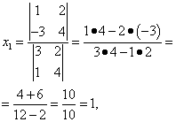
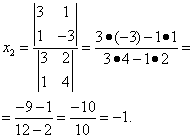
So, the solution of system (2):
online calculator, Cramer's solution method.
Three cases in solving systems of linear equations
As appears from Cramer's theorems, when solving a system of linear equations, three cases may occur:

First case: the system of linear equations has a unique solution
(the system is consistent and definite)

Second case: the system of linear equations has an infinite number of solutions
(the system is consistent and indeterminate)
** ![]() ,
,
those. the coefficients of the unknowns and the free terms are proportional.

Third case: the system of linear equations has no solutions
(system inconsistent)
So the system m linear equations with n variables is called incompatible if it has no solutions, and joint if it has at least one solution. A joint system of equations that has only one solution is called certain, and more than one uncertain.
Examples of solving systems of linear equations by the Cramer method
Let the system
 .
.
Based on Cramer's theorem
………….
,
where  -
-
system identifier. The remaining determinants are obtained by replacing the column with the coefficients of the corresponding variable (unknown) with free members:


Example 2
 .
.

Therefore, the system is definite. To find its solution, we calculate the determinants


By Cramer's formulas we find:
![]()
So, (1; 0; -1) is the only solution to the system.
To check the solutions of systems of equations 3 X 3 and 4 X 4, you can use the online calculator, the Cramer solving method.
If there are no variables in the system of linear equations in one or more equations, then in the determinant the elements corresponding to them are equal to zero! This is the next example.
Example 3 Solve the system of linear equations by Cramer's method:
 .
.
Solution. We find the determinant of the system:

Look carefully at the system of equations and at the determinant of the system and repeat the answer to the question in which cases one or more elements of the determinant are equal to zero. So, the determinant is not equal to zero, therefore, the system is definite. To find its solution, we calculate the determinants for the unknowns


By Cramer's formulas we find:
So, the solution of the system is (2; -1; 1).
To check the solutions of systems of equations 3 X 3 and 4 X 4, you can use the online calculator, the Cramer solving method.
Top of page
We continue to solve systems using the Cramer method together
As already mentioned, if the determinant of the system is equal to zero, and the determinants for the unknowns are not equal to zero, the system is inconsistent, that is, it has no solutions. Let's illustrate with the following example.
Example 6 Solve the system of linear equations by Cramer's method:

Solution. We find the determinant of the system:
The determinant of the system is equal to zero, therefore, the system of linear equations is either inconsistent and definite, or inconsistent, that is, it has no solutions. To clarify, we calculate the determinants for the unknowns


The determinants for the unknowns are not equal to zero, therefore, the system is inconsistent, that is, it has no solutions.
To check the solutions of systems of equations 3 X 3 and 4 X 4, you can use the online calculator, the Cramer solving method.
In problems on systems of linear equations, there are also those where, in addition to the letters denoting variables, there are also other letters. These letters stand for some number, most often a real number. In practice, such equations and systems of equations lead to problems to find the general properties of any phenomena and objects. That is, you invented some new material or device, and to describe its properties, which are common regardless of the size or number of copies, you need to solve a system of linear equations, where instead of some coefficients for variables there are letters. You don't have to look far for examples.
The next example is for a similar problem, only the number of equations, variables, and letters denoting some real number increases.
Example 8 Solve the system of linear equations by Cramer's method:
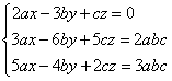
Solution. We find the determinant of the system:
Finding determinants for unknowns

KOSTROMA BRANCH OF THE MILITARY UNIVERSITY OF RCHB PROTECTION
Department of "Automation of command and control"
Only for teachers
"I approve"
Head of Department No. 9
Colonel YAKOVLEV A.B.
"____" ______________ 2004
Associate Professor A.I. Smirnova
"DETERMINERS.
SOLUTION OF SYSTEMS OF LINEAR EQUATIONS"
LECTURE № 2 / 1
Discussed at the meeting of the department No. 9
"____" ___________ 2004
Protocol No. ___________
Kostroma, 2004.
Introduction
1. Determinants of the second and third order.
2. Properties of determinants. Decomposition theorem.
3. Cramer's theorem.
Conclusion
Literature
1. V.E. Schneider et al., A Short Course in Higher Mathematics, Volume I, Ch. 2, item 1.
2. V.S. Shchipachev, Higher Mathematics, ch.10, p.2.
INTRODUCTION
The lecture deals with determinants of the second and third orders, their properties. As well as Cramer's theorem, which allows solving systems of linear equations using determinants. Determinants are also used later in the topic "Vector Algebra" when calculating the cross product of vectors.
1st study question QUALIFIERS OF THE SECOND AND THIRD
ORDER
Consider a table of four numbers of the form
The numbers in the table are denoted by a letter with two indices. The first index indicates the row number, the second index indicates the column number.
DEFINITION 1.Second order determinant calledexpressionkind:
(1)Numbers a 11, …, a 22 are called the elements of the determinant.
Diagonal formed by elements a 11 ; a 22 is called the main, and the diagonal formed by the elements a 12 ; a 21 - on the side.
Thus, the second-order determinant is equal to the difference between the products of the elements of the main and secondary diagonals.
Note that the answer is a number.
EXAMPLES. Calculate:
Consider now a table of nine numbers written in three rows and three columns:
DEFINITION 2. Third order determinant is called an expression of the form:
Elements a 11; a 22 ; a 33 - form the main diagonal.
Numbers a 13; a 22 ; a 31 - form a side diagonal.
Let us depict, schematically, how the terms with plus and minus are formed:
" + " " – "Plus includes: the product of the elements on the main diagonal, the other two terms are the product of the elements located at the vertices of triangles with bases parallel to the main diagonal.
Terms with a minus are formed in the same way with respect to the secondary diagonal.
This rule for calculating the third order determinant is called
right
EXAMPLES. Calculate by the rule of triangles:
COMMENT. Determinants are also called determinants.
2nd study question PROPERTIES OF DETERMINERS.
EXPANSION THEOREM
Property 1. The value of the determinant will not change if its rows are interchanged with the corresponding columns.
.Expanding both determinants, we are convinced of the validity of equality.
Property 1 sets the equality of rows and columns of the determinant. Therefore, all further properties of the determinant will be formulated for both rows and columns.
Property 2. When two rows (or columns) are interchanged, the determinant changes sign to the opposite, preserving the absolute value.
.Property 3. Common multiplier of row elements(or column)can be taken out of the sign of the determinant.
.Property 4. If the determinant has two identical rows (or columns), then it is equal to zero.
This property can be proved by direct verification, or property 2 can be used.
Denote the determinant by D. When two identical first and second rows are interchanged, it will not change, and by the second property it must change sign, i.e.
D = - DÞ 2 D = 0 ÞD = 0.
Property 5. If all elements of some string(or column)are zero, then the determinant is zero.
This property can be considered as a special case of property 3 with
Property 6. If the elements of two rows(or columns)determinant are proportional, then the determinant is zero.
.It can be proved by direct verification or by using properties 3 and 4.
Property 7. The value of the determinant does not change if the elements of any row (or column) are added to the corresponding elements of another row (or column), multiplied by the same number.
.It is proved by direct verification.
The use of these properties can in some cases facilitate the process of calculating determinants, especially of the third order.
For what follows, we need the concepts of minor and algebraic complement. Consider these concepts to define the third order.
DEFINITION 3. Minor of a given element of a third-order determinant is called a second-order determinant obtained from a given one by deleting the row and column at the intersection of which the given element stands.
Element minor aij denoted Mij. So for element a 11 minor
It is obtained by deleting the first row and the first column in the third-order determinant.
DEFINITION 4. Algebraic complement of the determinant element call it a minor multiplied by(-1)k, wherek- the sum of the row and column numbers at the intersection of which the given element is located.
Algebraic element addition aij denoted BUTij.
In this way, BUTij =
.Let us write out the algebraic complements for the elements a 11 and a 12.
. .It is useful to remember the rule: the algebraic complement of an element of a determinant is equal to its signed minor a plus, if the sum of the row and column numbers in which the element is located, even, and with sign minus if this amount odd.
EXAMPLE. Find minors and algebraic complements for elements of the first row of the determinant:
It is clear that minors and algebraic complements can differ only in sign.
Let us consider without proof an important theorem - the determinant expansion theorem.
EXPANSION THEOREM
The determinant is equal to the sum of the products of the elements of any row or column and their algebraic complements.
Using this theorem, we write the expansion of the third-order determinant in the first row.
.Expanded:
.The last formula can be used as the main one when calculating the third order determinant.
The decomposition theorem allows us to reduce the calculation of the third order determinant to the calculation of three second order determinants.
The decomposition theorem gives a second way to calculate third-order determinants.
EXAMPLES. Calculate the determinant using the expansion theorem.
Solving systems of linear algebraic equations (SLAE) is undoubtedly the most important topic of the linear algebra course. A huge number of problems from all branches of mathematics are reduced to solving systems of linear equations. These factors explain the reason for creating this article. The material of the article is selected and structured so that with its help you can
- choose the optimal method for solving your system of linear algebraic equations,
- study the theory of the chosen method,
- solve your system of linear equations, having considered in detail the solutions of typical examples and problems.
Brief description of the material of the article.
First, we give all the necessary definitions, concepts, and introduce some notation.
Next, we consider methods for solving systems of linear algebraic equations in which the number of equations is equal to the number of unknown variables and which have a unique solution. First, let's focus on the Cramer method, secondly, we will show the matrix method for solving such systems of equations, and thirdly, we will analyze the Gauss method (the method of successive elimination of unknown variables). To consolidate the theory, we will definitely solve several SLAEs in various ways.
After that, we turn to solving systems of linear algebraic equations of a general form, in which the number of equations does not coincide with the number of unknown variables or the main matrix of the system is degenerate. We formulate the Kronecker-Capelli theorem, which allows us to establish the compatibility of SLAEs. Let us analyze the solution of systems (in the case of their compatibility) using the concept of the basis minor of a matrix. We will also consider the Gauss method and describe in detail the solutions of the examples.
Be sure to dwell on the structure of the general solution of homogeneous and inhomogeneous systems of linear algebraic equations. Let us give the concept of a fundamental system of solutions and show how the general solution of the SLAE is written using the vectors of the fundamental system of solutions. For a better understanding, let's look at a few examples.
In conclusion, we consider systems of equations that are reduced to linear ones, as well as various problems, in the solution of which SLAEs arise.
Page navigation.
Definitions, concepts, designations.
We will consider systems of p linear algebraic equations with n unknown variables (p may be equal to n ) of the form
Unknown variables, - coefficients (some real or complex numbers), - free members (also real or complex numbers).
This form of SLAE is called coordinate.
AT matrix form this system of equations has the form ,
where  - the main matrix of the system, - the matrix-column of unknown variables, - the matrix-column of free members.
If we add to the matrix A as the (n + 1)-th column the matrix-column of free terms, then we get the so-called expanded matrix systems of linear equations. Usually, the augmented matrix is denoted by the letter T, and the column of free members is separated by a vertical line from the rest of the columns, that is, 
By solving a system of linear algebraic equations called a set of values of unknown variables , which turns all the equations of the system into identities. The matrix equation for the given values of the unknown variables also turns into an identity.
If a system of equations has at least one solution, then it is called joint.
If the system of equations has no solutions, then it is called incompatible.
If a SLAE has a unique solution, then it is called certain; if there is more than one solution, then - uncertain.
If the free terms of all equations of the system are equal to zero ![]() , then the system is called homogeneous, otherwise - heterogeneous.
, then the system is called homogeneous, otherwise - heterogeneous.
Solution of elementary systems of linear algebraic equations.
If the number of system equations is equal to the number of unknown variables and the determinant of its main matrix is not equal to zero, then we will call such SLAEs elementary. Such systems of equations have a unique solution, and in the case of a homogeneous system, all unknown variables are equal to zero.
We started studying such SLAE in high school. When solving them, we took one equation, expressed one unknown variable in terms of others and substituted it into the remaining equations, then took the next equation, expressed the next unknown variable and substituted it into other equations, and so on. Or they used the addition method, that is, they added two or more equations to eliminate some unknown variables. We will not dwell on these methods in detail, since they are essentially modifications of the Gauss method.
The main methods for solving elementary systems of linear equations are the Cramer method, the matrix method and the Gauss method. Let's sort them out.
Solving systems of linear equations by Cramer's method.
Let us need to solve a system of linear algebraic equations 
in which the number of equations is equal to the number of unknown variables and the determinant of the main matrix of the system is different from zero, that is, .
Let be the determinant of the main matrix of the system, and ![]() are determinants of matrices that are obtained from A by replacing 1st, 2nd, …, nth column respectively to the column of free members:
are determinants of matrices that are obtained from A by replacing 1st, 2nd, …, nth column respectively to the column of free members: 
With such notation, the unknown variables are calculated by the formulas of Cramer's method as  . This is how the solution of a system of linear algebraic equations is found by the Cramer method.
Example.
Cramer method  .
.
Solution.
The main matrix of the system has the form  . Calculate its determinant (if necessary, see the article):
Since the determinant of the main matrix of the system is nonzero, the system has a unique solution that can be found by Cramer's method.
Compose and calculate the necessary determinants ![]() (the determinant is obtained by replacing the first column in matrix A with a column of free members, the determinant - by replacing the second column with a column of free members, - by replacing the third column of matrix A with a column of free members):
(the determinant is obtained by replacing the first column in matrix A with a column of free members, the determinant - by replacing the second column with a column of free members, - by replacing the third column of matrix A with a column of free members): 
Finding unknown variables using formulas  :
:
Answer:
The main disadvantage of Cramer's method (if it can be called a disadvantage) is the complexity of calculating the determinants when the number of system equations is more than three.
Solving systems of linear algebraic equations by the matrix method (using the inverse matrix).
Let the system of linear algebraic equations be given in matrix form , where the matrix A has dimension n by n and its determinant is nonzero.
Since , then the matrix A is invertible, that is, there is an inverse matrix . If we multiply both parts of the equality by on the left, then we get a formula for finding the column matrix of unknown variables. So we got the solution of the system of linear algebraic equations by the matrix method.
Example.
Solve System of Linear Equations matrix method.
Solution.
Let's rewrite the system of equations in matrix form: 
Because
then the SLAE can be solved by the matrix method. Using the inverse matrix, the solution to this system can be found as  .
.
Let's build an inverse matrix using a matrix of algebraic complements of the elements of matrix A (if necessary, see the article): 
It remains to calculate - the matrix of unknown variables by multiplying the inverse matrix  on the matrix-column of free members (if necessary, see the article):
Answer:
 or in another notation x 1 = 4, x 2 = 0, x 3 = -1.
The main problem in finding solutions to systems of linear algebraic equations by the matrix method is the complexity of finding the inverse matrix, especially for square matrices of order higher than the third.
Solving systems of linear equations by the Gauss method.
Suppose we need to find a solution to a system of n linear equations with n unknown variables 
the determinant of the main matrix of which is different from zero.
The essence of the Gauss method consists in the successive exclusion of unknown variables: first, x 1 is excluded from all equations of the system, starting from the second, then x 2 is excluded from all equations, starting from the third, and so on, until only the unknown variable x n remains in the last equation. Such a process of transforming the equations of the system for the successive elimination of unknown variables is called direct Gauss method. After the completion of the forward run of the Gaussian method, x n is found from the last equation, x n-1 is calculated from the penultimate equation using this value, and so on, x 1 is found from the first equation. The process of calculating unknown variables when moving from the last equation of the system to the first is called reverse Gauss method.
Let us briefly describe the algorithm for eliminating unknown variables.
We will assume that , since we can always achieve this by rearranging the equations of the system. We exclude the unknown variable x 1 from all equations of the system, starting from the second one. To do this, add the first equation multiplied by to the second equation of the system, add the first multiplied by to the third equation, and so on, add the first multiplied by to the nth equation. The system of equations after such transformations will take the form 
where , a  .
.
We would come to the same result if we expressed x 1 in terms of other unknown variables in the first equation of the system and substituted the resulting expression into all other equations. Thus, the variable x 1 is excluded from all equations, starting from the second.
Next, we act similarly, but only with a part of the resulting system, which is marked in the figure 
To do this, add the second multiplied by to the third equation of the system, add the second multiplied by to the fourth equation, and so on, add the second multiplied by to the nth equation. The system of equations after such transformations will take the form 
where , a  . Thus, the variable x 2 is excluded from all equations, starting from the third.
Next, we proceed to the elimination of the unknown x 3, while acting similarly with the part of the system marked in the figure 
So we continue the direct course of the Gauss method until the system takes the form 
From this moment, we begin the reverse course of the Gauss method: we calculate x n from the last equation as , using the obtained value x n we find x n-1 from the penultimate equation, and so on, we find x 1 from the first equation.
Example.
Solve System of Linear Equations Gaussian method.
Solution.
Let's exclude the unknown variable x 1 from the second and third equations of the system. To do this, to both parts of the second and third equations, we add the corresponding parts of the first equation, multiplied by and by, respectively: 
Now we exclude x 2 from the third equation by adding to its left and right parts the left and right parts of the second equation, multiplied by: 
On this, the forward course of the Gauss method is completed, we begin the reverse course.
From the last equation of the resulting system of equations, we find x 3: 
From the second equation we get .
From the first equation we find the remaining unknown variable and this completes the reverse course of the Gauss method.
Answer:
X 1 \u003d 4, x 2 \u003d 0, x 3 \u003d -1.
Solving systems of linear algebraic equations of general form.
In the general case, the number of equations of the system p does not coincide with the number of unknown variables n:
Such SLAEs may have no solutions, have a single solution, or have infinitely many solutions. This statement also applies to systems of equations whose main matrix is square and degenerate.
Kronecker-Capelli theorem.
Before finding a solution to a system of linear equations, it is necessary to establish its compatibility. The answer to the question when SLAE is compatible, and when it is incompatible, gives Kronecker–Capelli theorem:
for a system of p equations with n unknowns (p can be equal to n ) to be consistent it is necessary and sufficient that the rank of the main matrix of the system is equal to the rank of the extended matrix, that is, Rank(A)=Rank(T) .
Let us consider the application of the Kronecker-Cappelli theorem for determining the compatibility of a system of linear equations as an example.
Example.
Find out if the system of linear equations has  solutions.
Solution.
 . Let us use the method of bordering minors. Minor of the second order
  different from zero. Let's go over the third-order minors surrounding it:
Since all bordering third-order minors are equal to zero, the rank of the main matrix is two.
In turn, the rank of the augmented matrix  is equal to three, since the minor of the third order
different from zero.
In this way, Rang(A) , therefore, according to the Kronecker-Capelli theorem, we can conclude that the original system of linear equations is inconsistent.
Answer:
There is no solution system.
So, we have learned to establish the inconsistency of the system using the Kronecker-Capelli theorem.
But how to find the solution of the SLAE if its compatibility is established?
To do this, we need the concept of the basis minor of a matrix and the theorem on the rank of a matrix.
The highest order minor of the matrix A, other than zero, is called basic.
It follows from the definition of the basis minor that its order is equal to the rank of the matrix. For a non-zero matrix A, there can be several basic minors; there is always one basic minor.
For example, consider the matrix  .
.
All third-order minors of this matrix are equal to zero, since the elements of the third row of this matrix are the sum of the corresponding elements of the first and second rows.
The following minors of the second order are basic, since they are nonzero 
Minors  are not basic, since they are equal to zero.
Matrix rank theorem.
If the rank of a matrix of order p by n is r, then all elements of the rows (and columns) of the matrix that do not form the chosen basis minor are linearly expressed in terms of the corresponding elements of the rows (and columns) that form the basis minor.
What does the matrix rank theorem give us?
If, by the Kronecker-Capelli theorem, we have established the compatibility of the system, then we choose any basic minor of the main matrix of the system (its order is equal to r), and exclude from the system all equations that do not form the chosen basic minor. The SLAE obtained in this way will be equivalent to the original one, since the discarded equations are still redundant (according to the matrix rank theorem, they are a linear combination of the remaining equations).
As a result, after discarding the excessive equations of the system, two cases are possible.
If the number of equations r in the resulting system is equal to the number of unknown variables, then it will be definite and the only solution can be found by the Cramer method, the matrix method or the Gauss method.
Example.
 .
.
Solution.
Rank of the main matrix of the system  is equal to two, since the minor of the second order
  different from zero. Extended matrix rank
  is also equal to two, since the only minor of the third order is equal to zero
and the minor of the second order considered above is different from zero. Based on the Kronecker-Capelli theorem, one can assert the compatibility of the original system of linear equations, since Rank(A)=Rank(T)=2 .
As a basis minor, we take . It is formed by the coefficients of the first and second equations: 
The third equation of the system does not participate in the formation of the basic minor, so we exclude it from the system based on the matrix rank theorem: 
Thus we have obtained an elementary system of linear algebraic equations. Let's solve it by Cramer's method: 
Answer:
x 1 \u003d 1, x 2 \u003d 2.
If the number of equations r in the resulting SLAE is less than the number of unknown variables n , then we leave the terms that form the basic minor in the left parts of the equations, and transfer the remaining terms to the right parts of the equations of the system with the opposite sign.
The unknown variables (there are r of them) remaining on the left-hand sides of the equations are called main.
Unknown variables (there are n - r of them) that ended up on the right side are called free.
Now we assume that the free unknown variables can take arbitrary values, while the r main unknown variables will be expressed in terms of the free unknown variables in a unique way. Their expression can be found by solving the resulting SLAE by the Cramer method, the matrix method, or the Gauss method.
Let's take an example.
Example.
Solve System of Linear Algebraic Equations  .
.
Solution.
Find the rank of the main matrix of the system  by the bordering minors method. Let us take a 1 1 = 1 as a non-zero first-order minor. Let's start searching for a non-zero second-order minor surrounding this minor:
So we found a non-zero minor of the second order. Let's start searching for a non-zero bordering minor of the third order: 
Thus, the rank of the main matrix is three. The rank of the augmented matrix is also equal to three, that is, the system is consistent.
The found non-zero minor of the third order will be taken as the basic one.
For clarity, we show the elements that form the basis minor: 
We leave the terms participating in the basic minor on the left side of the equations of the system, and transfer the rest with opposite signs to the right sides: 
We give free unknown variables x 2 and x 5 arbitrary values, that is, we take ![]() , where are arbitrary numbers. In this case, the SLAE takes the form
, where are arbitrary numbers. In this case, the SLAE takes the form 
We solve the obtained elementary system of linear algebraic equations by the Cramer method: 
Consequently, .
In the answer, do not forget to indicate free unknown variables.
Answer:
Where are arbitrary numbers.
Summarize.
To solve a system of linear algebraic equations of a general form, we first find out its compatibility using the Kronecker-Capelli theorem. If the rank of the main matrix is not equal to the rank of the extended matrix, then we conclude that the system is inconsistent.
If the rank of the main matrix is equal to the rank of the extended matrix, then we choose the basic minor and discard the equations of the system that do not participate in the formation of the chosen basic minor.
If the order of the basis minor is equal to the number of unknown variables, then the SLAE has a unique solution, which can be found by any method known to us.
If the order of the basis minor is less than the number of unknown variables, then we leave the terms with the main unknown variables on the left side of the equations of the system, transfer the remaining terms to the right sides and assign arbitrary values to the free unknown variables. From the resulting system of linear equations, we find the main unknown variables by the Cramer method, the matrix method or the Gauss method.
Gauss method for solving systems of linear algebraic equations of general form.
Using the Gauss method, one can solve systems of linear algebraic equations of any kind without their preliminary investigation for compatibility. The process of successive elimination of unknown variables makes it possible to draw a conclusion about both the compatibility and inconsistency of the SLAE, and if a solution exists, it makes it possible to find it.
From the point of view of computational work, the Gaussian method is preferable.
See its detailed description and analyzed examples in the article Gauss method for solving systems of linear algebraic equations of general form.
Recording the general solution of homogeneous and inhomogeneous linear algebraic systems using the vectors of the fundamental system of solutions.
In this section, we will focus on joint homogeneous and inhomogeneous systems of linear algebraic equations that have an infinite number of solutions.
Let's deal with homogeneous systems first.
Fundamental decision system A homogeneous system of p linear algebraic equations with n unknown variables is a set of (n – r) linearly independent solutions of this system, where r is the order of the basis minor of the main matrix of the system.
If we designate linearly independent solutions of a homogeneous SLAE as X (1) , X (2) , …, X (n-r) (X (1) , X (2) , …, X (n-r) are matrices columns of dimension n by 1 ) , then the general solution of this homogeneous system is represented as a linear combination of vectors of the fundamental system of solutions with arbitrary constant coefficients С 1 , С 2 , …, С (n-r), that is, .
What does the term general solution of a homogeneous system of linear algebraic equations (oroslau) mean?
The meaning is simple: the formula specifies all possible solutions to the original SLAE, in other words, taking any set of values of arbitrary constants C 1 , C 2 , ..., C (n-r) , according to the formula we will get one of the solutions of the original homogeneous SLAE.
Thus, if we find a fundamental system of solutions, then we can set all solutions of this homogeneous SLAE as .
Let us show the process of constructing a fundamental system of solutions for a homogeneous SLAE.
We choose the basic minor of the original system of linear equations, exclude all other equations from the system, and transfer to the right-hand side of the equations of the system with opposite signs all terms containing free unknown variables. Let's give the free unknown variables the values 1,0,0,…,0 and calculate the main unknowns by solving the resulting elementary system of linear equations in any way, for example, by the Cramer method. Thus, X (1) will be obtained - the first solution of the fundamental system. If we give the free unknowns the values 0,1,0,0,…,0 and calculate the main unknowns, then we get X (2) . And so on. If we give the free unknown variables the values 0,0,…,0,1 and calculate the main unknowns, then we get X (n-r) . This is how the fundamental system of solutions of the homogeneous SLAE will be constructed and its general solution can be written in the form .
For inhomogeneous systems of linear algebraic equations, the general solution is represented as
Let's look at examples.
Example.
Find the fundamental system of solutions and the general solution of a homogeneous system of linear algebraic equations  .
.
Solution.
The rank of the main matrix of homogeneous systems of linear equations is always equal to the rank of the extended matrix. Let us find the rank of the main matrix by the method of fringing minors. As a nonzero minor of the first order, we take the element a 1 1 = 9 of the main matrix of the system. Find the bordering non-zero minor of the second order: 
A minor of the second order, different from zero, is found. Let's go through the third-order minors bordering it in search of a non-zero one: 
All bordering minors of the third order are equal to zero, therefore, the rank of the main and extended matrix is two. Let's take the basic minor. For clarity, we note the elements of the system that form it: 
The third equation of the original SLAE does not participate in the formation of the basic minor, therefore, it can be excluded: 
We leave the terms containing the main unknowns on the right-hand sides of the equations, and transfer the terms with free unknowns to the right-hand sides:
Let us construct a fundamental system of solutions to the original homogeneous system of linear equations. The fundamental system of solutions of this SLAE consists of two solutions, since the original SLAE contains four unknown variables, and the order of its basic minor is two. To find X (1), we give the free unknown variables the values x 2 \u003d 1, x 4 \u003d 0, then we find the main unknowns from the system of equations  .
.
Let's solve it by Cramer's method: 
In this way, .
Now let's build X (2) . To do this, we give the free unknown variables the values x 2 \u003d 0, x 4 \u003d 1, then we find the main unknowns from the system of linear equations  .
.
Let's use Cramer's method again: 
We get .
So we got two vectors of the fundamental system of solutions and , now we can write down the general solution of a homogeneous system of linear algebraic equations:  , where C 1 and C 2 are arbitrary numbers., are equal to zero. We also take the minor as the basic one, exclude the third equation from the system, and transfer the terms with free unknowns to the right-hand sides of the system equations:
To find, we give the free unknown variables the values x 2 \u003d 0 and x 4 \u003d 0, then the system of equations takes the form  , from which we find the main unknown variables using the Cramer method:
We have  , Consequently,
where C 1 and C 2 are arbitrary numbers.
It should be noted that the solutions of an indefinite homogeneous system of linear algebraic equations generate linear space Solution.
The canonical equation of an ellipsoid in a rectangular Cartesian coordinate system has the form  . Our task is to determine the parameters a , b and c . Since the ellipsoid passes through points A, B and C, then when substituting their coordinates into the canonical equation of the ellipsoid, it should turn into an identity. So we get a system of three equations:
Denote ![]() , then the system becomes a system of linear algebraic equations
, then the system becomes a system of linear algebraic equations  .
.
Let us calculate the determinant of the main matrix of the system: 
Since it is non-zero, we can find the solution by Cramer's method:
). Obviously, x = 0 and x = 1 are the roots of this polynomial. quotient from division ![]() on the
on the ![]() is . Thus, we have a decomposition and the original expression will take the form
is . Thus, we have a decomposition and the original expression will take the form  .
.
Let's use the method of indefinite coefficients. 
Equating the corresponding coefficients of the numerators, we arrive at a system of linear algebraic equations  . Its solution will give us the desired indefinite coefficients A, B, C and D.
We solve the system using the Gauss method: 
In the reverse course of the Gauss method, we find D = 0, C = -2, B = 1, A = 1 .
We get 
Answer:
 .
.