Find the determinant of the original matrix. If the determinant of a matrix is ​​zero, then its inverse does not exist.

Formulation of the problem

The task involves familiarizing the user with the basic concepts of numerical methods, such as determinant and inverse matrix, and various ways to calculate them. In this theoretical report, in simple and accessible language, the basic concepts and definitions are first introduced, on the basis of which further research is carried out. The user may not have special knowledge in the field of numerical methods and linear algebra, but will easily be able to use the results of this work. For clarity, a program for calculating the matrix determinant by several methods, written in the C ++ programming language, is given. The program is used as a laboratory stand for creating illustrations for the report. And also a study of methods for solving systems of linear algebraic equations is being carried out. The uselessness of calculating the inverse matrix is ​​proved, so the paper provides more optimal ways to solve equations without calculating it. It is explained why there are so many different methods for calculating determinants and inverse matrices and their shortcomings are analyzed. Errors in the calculation of the determinant are also considered and the achieved accuracy is estimated. In addition to Russian terms, their English equivalents are also used in the work to understand under what names to search for numerical procedures in libraries and what their parameters mean.

Basic definitions and simple properties

Determinant

Let us introduce the definition of the determinant of a square matrix of any order. This definition will recurrent, that is, to establish what the determinant of the order matrix is, you need to already know what the determinant of the order matrix is. Note also that the determinant exists only for square matrices.

The determinant of a square matrix will be denoted by or det .

Definition 1. determinant square matrix second order number is called .

determinant square matrix of order , is called the number

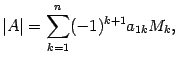
where is the determinant of the order matrix obtained from the matrix by deleting the first row and the column with the number .

For clarity, we write down how you can calculate the determinant of a matrix of the fourth order:

Comment. The actual calculation of determinants for matrices above the third order based on the definition is used in exceptional cases. As a rule, the calculation is carried out according to other algorithms, which will be discussed later and which require less computational work.

Comment. In Definition 1, it would be more accurate to say that the determinant is a function defined on the set of square order matrices and taking values ​​in the set of numbers.

Comment. In the literature, instead of the term "determinant", the term "determinant" is also used, which has the same meaning. From the word "determinant" the designation det appeared.

Let us consider some properties of determinants, which we formulate in the form of assertions.

Statement 1. When transposing a matrix, the determinant does not change, that is, .

Statement 2. The determinant of the product of square matrices is equal to the product of the determinants of the factors, that is, .

Statement 3. If two rows in a matrix are swapped, then its determinant will change sign.

Statement 4. If a matrix has two identical rows, then its determinant is zero.

In the future, we will need to add strings and multiply a string by a number. We will perform these operations on rows (columns) in the same way as operations on row matrices (column matrices), that is, element by element. The result will be a row (column), which, as a rule, does not match the rows of the original matrix. In the presence of operations of adding rows (columns) and multiplying them by a number, we can also talk about linear combinations of rows (columns), that is, sums with numerical coefficients.

Statement 5. If a row of a matrix is ​​multiplied by a number, then its determinant will be multiplied by that number.

Statement 6. If the matrix contains a zero row, then its determinant is zero.

Statement 7. If one of the rows of the matrix is ​​equal to the other multiplied by a number (the rows are proportional), then the determinant of the matrix is ​​zero.

Statement 8. Let the i-th row in the matrix look like . Then , where the matrix is ​​obtained from the matrix by replacing the i-th row with the row , and the matrix is ​​obtained by replacing the i-th row with the row .

Statement 9. If one of the rows of the matrix is ​​added to another, multiplied by a number, then the determinant of the matrix will not change.

Statement 10. If one of the rows of a matrix is ​​a linear combination of its other rows, then the determinant of the matrix is ​​zero.

Definition 2. Algebraic addition to a matrix element is called a number equal to , where is the determinant of the matrix obtained from the matrix by deleting the i-th row and the j-th column. The algebraic complement to a matrix element is denoted by .

Example. Let 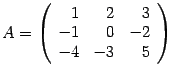. Then

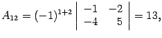
Comment. Using algebraic additions, the definition of 1 determinant can be written as follows: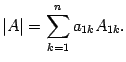

Statement 11. Decomposition of the determinant in an arbitrary string.

The matrix determinant satisfies the formula

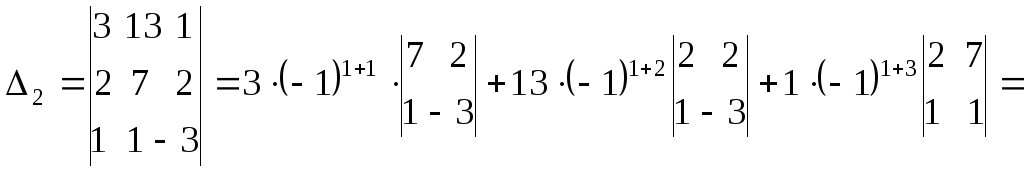
Example. Calculate .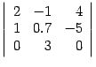

Solution. Let's use the expansion in the third line, it's more profitable, because in the third line two numbers out of three are zeros. Get

Statement 12. For a square matrix of order at , we have the relation .

Statement 13. All properties of the determinant formulated for rows (statements 1 - 11) are also valid for columns, in particular, the expansion of the determinant in the j-th column is valid 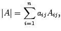and equality at .

Statement 14. The determinant of a triangular matrix is ​​equal to the product of the elements of its main diagonal.

Consequence. The determinant of the identity matrix is ​​equal to one, .

Conclusion. The properties listed above make it possible to find determinants of matrices of sufficiently high orders with a relatively small amount of calculations. The calculation algorithm is the following.

Algorithm for creating zeros in a column. Let it be required to calculate the order determinant . If , then swap the first line and any other line in which the first element is not zero. As a result, the determinant , will be equal to the determinant of the new matrix with the opposite sign. If the first element of each row is equal to zero, then the matrix has a zero column and, by Statements 1, 13, its determinant is equal to zero.

So, we consider that already in the original matrix . Leave the first line unchanged. Let's add to the second line the first line, multiplied by the number . Then the first element of the second row will be equal to .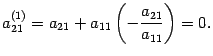

The remaining elements of the new second row will be denoted by , . The determinant of the new matrix according to Statement 9 is equal to . Multiply the first line by the number and add it to the third. The first element of the new third row will be equal to

The remaining elements of the new third row will be denoted by , . The determinant of the new matrix according to Statement 9 is equal to .

We will continue the process of obtaining zeros instead of the first elements of strings. Finally, we multiply the first line by a number and add it to the last line. The result is a matrix, denoted by , which has the form

and . To calculate the determinant of the matrix, we use the expansion in the first column

Since then

The determinant of the order matrix is ​​on the right side. We apply the same algorithm to it, and the calculation of the determinant of the matrix will be reduced to the calculation of the determinant of the order matrix. The process is repeated until we reach the second-order determinant, which is calculated by definition.

If the matrix does not have any specific properties, then it is not possible to significantly reduce the amount of calculations compared to the proposed algorithm. Another good side of this algorithm is that it is easy to write a program for a computer to calculate the determinants of matrices of large orders. In standard programs for calculating determinants, this algorithm is used with minor changes associated with minimizing the effect of rounding errors and input data errors in computer calculations.

Example. Compute Matrix Determinant .

Solution. The first line is left unchanged. To the second line we add the first, multiplied by the number:

The determinant does not change. To the third line we add the first, multiplied by the number:

The determinant does not change. To the fourth line we add the first, multiplied by the number:

The determinant does not change. As a result, we get

Using the same algorithm, we calculate the determinant of a matrix of order 3, which is on the right. We leave the first line unchanged, to the second line we add the first, multiplied by the number :

To the third line we add the first, multiplied by the number :

As a result, we get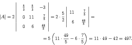

Answer. .

Comment. Although fractions were used in the calculations, the result was an integer. Indeed, using the properties of determinants and the fact that the original numbers are integers, operations with fractions could be avoided. But in engineering practice, numbers are extremely rarely integers. Therefore, as a rule, the elements of the determinant will be decimal fractions and it is not advisable to use any tricks to simplify calculations.

inverse matrix

Definition 3. The matrix is ​​called inverse matrix for a square matrix if .

It follows from the definition that the inverse matrix will be a square matrix of the same order as the matrix (otherwise one of the products or would not be defined).

The inverse matrix for a matrix is ​​denoted by . Thus, if exists, then .

From the definition of an inverse matrix, it follows that the matrix is ​​the inverse of the matrix, that is, . Matrices and can be said to be inverse to each other or mutually inverse.

If the determinant of a matrix is ​​zero, then its inverse does not exist.

Since for finding the inverse matrix it is important whether the determinant of the matrix is ​​equal to zero or not, we introduce the following definitions.

Definition 4. Let's call the square matrix degenerate or special matrix, if and non-degenerate or nonsingular matrix, if .

Statement. If an inverse matrix exists, then it is unique.

Statement. If a square matrix is ​​nondegenerate, then its inverse exists and 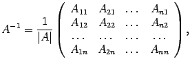(1) where are algebraic additions to elements .

Theorem. An inverse matrix for a square matrix exists if and only if the matrix is ​​nonsingular, the inverse matrix is ​​unique, and formula (1) is valid.

Comment. Particular attention should be paid to the places occupied by algebraic additions in the inverse matrix formula: the first index shows the number column, and the second is the number lines, in which the calculated algebraic complement should be written.

Example. .

Solution. Finding the determinant

Since , then the matrix is ​​nondegenerate, and the inverse for it exists. Finding algebraic additions:

We compose the inverse matrix by placing the found algebraic additions so that the first index corresponds to the column, and the second to the row: (2)

The resulting matrix (2) is the answer to the problem.

Comment. In the previous example, it would be more accurate to write the answer like this:
(3)

However, the notation (2) is more compact and it is more convenient to carry out further calculations, if any, with it. Therefore, writing the answer in the form (2) is preferable if the elements of the matrices are integers. And vice versa, if the elements of the matrix are decimal fractions, then it is better to write the inverse matrix without a factor in front.

Comment. When finding the inverse matrix, you have to perform quite a lot of calculations and an unusual rule for arranging algebraic additions in the final matrix. Therefore, there is a high chance of error. To avoid errors, you should do a check: calculate the product of the original matrix by the final one in one order or another. If the result is an identity matrix, then the inverse matrix is ​​found correctly. Otherwise, you need to look for an error.

Example. Find the inverse of a matrix .

Solution. - exists.

Answer: .

Conclusion. Finding the inverse matrix by formula (1) requires too many calculations. For matrices of the fourth order and higher, this is unacceptable. The real algorithm for finding the inverse matrix will be given later.

Calculating the determinant and inverse matrix using the Gauss method

The Gauss method can be used to find the determinant and inverse matrix.

Namely, the matrix determinant is equal to det .

The inverse matrix is ​​found by solving systems of linear equations using the Gaussian elimination method:

Where is the j-th column of the identity matrix , is the desired vector.

The resulting solution vectors - form, obviously, the columns of the matrix, since .

Formulas for the determinant

1. If the matrix is ​​nonsingular, then and (the product of the leading elements).

A system of N linear algebraic equations (SLAE) with unknowns is given, the coefficients of which are the elements of the matrix , and the free members are the numbers

The first index next to the coefficients indicates in which equation the coefficient is located, and the second - at which of the unknowns it is located.

If the matrix determinant is not equal to zero

then the system of linear algebraic equations has a unique solution.

The solution of a system of linear algebraic equations is such an ordered set of numbers , which at turns each of the equations of the system into a correct equality.

If the right sides of all equations of the system are equal to zero, then the system of equations is called homogeneous. In the case when some of them are nonzero, non-uniform

If a system of linear algebraic equations has at least one solution, then it is called compatible, otherwise it is incompatible.

If the solution of the system is unique, then the system of linear equations is called definite. In the case when the solution of the joint system is not unique, the system of equations is called indefinite.

Two systems of linear equations are called equivalent (or equivalent) if all solutions of one system are solutions of the second, and vice versa. Equivalent (or equivalent) systems are obtained using equivalent transformations.

Equivalent transformations of SLAE

1) rearrangement of equations;

2) multiplication (or division) of equations by a non-zero number;

3) adding to some equation another equation, multiplied by an arbitrary non-zero number.

The SLAE solution can be found in different ways.

CRAMER'S METHOD

CRAMER'S THEOREM. If the determinant of a system of linear algebraic equations with unknowns is different from zero, then this system has a unique solution, which is found by the Cramer formulas:

are determinants formed with the replacement of the i-th column by a column of free members.

If , and at least one of is nonzero, then SLAE has no solutions. If , then the SLAE has many solutions. Consider examples using Cramer's method.

—————————————————————

A system of three linear equations with three unknowns is given. Solve the system by Cramer's method

Find the determinant of the matrix of coefficients for unknowns

Since , then the given system of equations is consistent and has a unique solution. Let's calculate the determinants:

Using Cramer's formulas, we find the unknowns

So the only solution to the system.

A system of four linear algebraic equations is given. Solve the system by Cramer's method.

Let us find the determinant of the matrix of coefficients for the unknowns. To do this, we expand it by the first line.

Find the components of the determinant:

Substitute the found values ​​into the determinant

The determinant, therefore, the system of equations is consistent and has a unique solution. We calculate the determinants using Cramer's formulas:

Let's expand each of the determinants by the column in which there are more zeros.

By Cramer's formulas we find

System Solution

This example can be solved with a mathematical calculator YukhymCALC. A fragment of the program and the results of calculations are shown below.

——————————

C R A M E R METHOD

|1,1,1,1|

D=|5,-3,2,-8|

|3,5,1,4|

|4,2,3,1|

D=1*(-3*1*1+2*4*2+(-8)*5*3-((-8)*1*2+2*5*1+(-3)*4* 3))-1*(5*1*1+2*4*4+(-8)*3*3-((-8)*1*4+2*3*1+5*4*3) )+1*(5*5*1+(-3)*4*4+(-8)*3*2-((-8)*5*4+(-3)*3*1+5* 4*2))-1*(5*1*1+2*4*4+(-8)*3*3-((-8)*1*4+2*3*1+5*4* 3))= 1*(-3+16-120+16-10+36)-1*(5+32-72+32-6-60)+1*(25-48-48+160+9- 40)-1*(75-12+12-40+27-10)=1*(-65)-1*(-69)+1*58-1*52=-65+69+58-52= ten

|0,1,1,1|

Dx1=|1,-3,2,-8|

|0,5,1,4|

|3,2,3,1|

Dx1=-1*(1*1*1+2*4*3+(-8)*0*3-((-8)*1*3+2*0*1+1*4*3)) +1*(1*5*1+(-3)*4*3+(-8)*0*2-((-8)*5*3+(-3)*0*1+1*4 *2))-1*(1*1*1+2*4*3+(-8)*0*3-((-8)*1*3+2*0*1+1*4*3 ))= -1*(1+24+0+24+0-12)+1*(5-36+0+120+0-8)-1*(15-9+0-30+0-2 )= -1*(37)+1*81-1*(-26)=-37+81+26=70

|1,0,1,1|

Dx2=|5,1,2,-8|

|3,0,1,4|

|4,3,3,1|

Dx2=1*(1*1*1+2*4*3+(-8)*0*3-((-8)*1*3+2*0*1+1*4*3))+ 1*(5*0*1+1*4*4+(-8)*3*3-((-8)*0*4+1*3*1+5*4*3))-1* (5*1*1+2*4*4+(-8)*3*3-((-8)*1*4+2*3*1+5*4*3))= 1*(1 +24+0+24+0-12)+1*(0+16-72+0-3-60)-1*(0+4+18+0-9-15)= 1*37+1* (-119)-1*(-2)=37-119+2=-80

|1,1,0,1|

Dx3=|5,-3,1,-8|

|3,5,0,4|

|4,2,3,1|

Dx3=1*(-3*0*1+1*4*2+(-8)*5*3-((-8)*0*2+1*5*1+(-3)*4* 3))-1*(5*0*1+1*4*4+(-8)*3*3-((-8)*0*4+1*3*1+5*4*3) )-1*(5*0*1+1*4*4+(-8)*3*3-((-8)*0*4+1*3*1+5*4*3))= 1*(0+8-120+0-5+36)-1*(0+16-72+0-3-60)-1*(75+0+6-20+27+0)= 1* (-81)-1*(-119)-1*88=-81+119-88=-50

|1,1,1,0|

Dx4=|5,-3,2,1|

|3,5,1,0|

|4,2,3,3|

Dx4=1*(-3*1*3+2*0*2+1*5*3-(1*1*2+2*5*3+(-3)*0*3))-1* (5*1*3+2*0*4+1*3*3-(1*1*4+2*3*3+5*0*3))+1*(5*5*3+( -3)*0*4+1*3*2-(1*5*4+(-3)*3*3+5*0*2))= 1*(-9+0+15-2- 30+0)-1*(15+0+9-4-18+0)+1*(75+0+6-20+27+0)= 1*(-26)-1*(2)+ 1*88=-26-2+88=60

x1=Dx1/D=70.0000/10.0000=7.0000

x2=Dx2/D=-80.0000/10.0000=-8.0000

x3=Dx3/D=-50.0000/10.0000=-5.0000

x4=Dx4/D=60.0000/10.0000=6.0000

View materials:

(jcomments on)

In the general case, the rule for computing determinants of the th order is rather cumbersome. For determinants of the second and third order, there are rational ways to calculate them.

Calculations of second-order determinants

To calculate the determinant of the matrix of the second order, it is necessary to subtract the product of the elements of the secondary diagonal from the product of the elements of the main diagonal:

Example

Exercise. Calculate second order determinant

Solution.

Answer.

Methods for calculating third-order determinants

There are rules for computing third-order determinants.

triangle rule

Schematically, this rule can be represented as follows:

The product of elements in the first determinant that are connected by lines is taken with a plus sign; similarly, for the second determinant, the corresponding products are taken with a minus sign, i.e.

Example

Exercise. Compute determinant triangle method.

Solution.

Answer.

Sarrus rule

To the right of the determinant, the first two columns are added and the products of the elements on the main diagonal and on the diagonals parallel to it are taken with a plus sign; and the products of the elements of the secondary diagonal and the diagonals parallel to it, with a minus sign:

Example

Exercise. Compute determinant using the Sarrus rule.

Solution.

Answer.

Row or column expansion of determinant

The determinant is equal to the sum of the products of the elements of the row of the determinant and their algebraic complements.

Usually choose the row/column in which/th there are zeros. The row or column on which the decomposition is carried out will be indicated by an arrow.

Example

Exercise. Expanding over the first row, calculate the determinant

Solution.

Answer.

This method allows the calculation of the determinant to be reduced to the calculation of a determinant of a lower order.

Example

Exercise. Compute determinant

Solution. Let us perform the following transformations on the rows of the determinant: from the second row we subtract the first four, and from the third row the first row multiplied by seven, as a result, according to the properties of the determinant, we obtain a determinant equal to the given one.

The determinant is zero because the second and third rows are proportional.

Answer.

To calculate the determinants of the fourth order and above, either expansion in a row / column, or reduction to a triangular form, or using Laplace's theorem is used.

Decomposition of the determinant in terms of the elements of a row or column

Example

Exercise. Compute determinant , decomposing it by the elements of some row or some column.

Solution. Let us first perform elementary transformations on the rows of the determinant by making as many zeros as possible either in a row or in a column. To do this, first we subtract nine thirds from the first line, five thirds from the second, and three thirds from the fourth, we get:

We expand the resulting determinant by the elements of the first column:

The resulting third-order determinant is also expanded by the elements of the row and column, having previously obtained zeros, for example, in the first column.

To do this, we subtract two second lines from the first line, and the second from the third:

Answer.

Comment

The last and penultimate determinants could not be calculated, but immediately conclude that they are equal to zero, since they contain proportional rows.

Bringing the determinant to a triangular form

With the help of elementary transformations over rows or columns, the determinant is reduced to a triangular form, and then its value, according to the properties of the determinant, is equal to the product of the elements on the main diagonal.

Example

Exercise. Compute determinant bringing it to a triangular shape.

Solution. First, we make zeros in the first column under the main diagonal.

4. Properties of determinants. Determinant of product of matrices.

All transformations will be easier to perform if the element is equal to 1. To do this, we will swap the first and second columns of the determinant, which, according to the properties of the determinant, will cause it to change sign to the opposite:

Next, we get zeros in the second column in place of the elements under the main diagonal. And again, if the diagonal element is equal to , then the calculations will be simpler. To do this, we swap the second and third lines (and at the same time change to the opposite sign of the determinant):

Answer.

Laplace's theorem

Example

Exercise. Using Laplace's theorem, calculate the determinant

Solution. We choose two rows in this fifth-order determinant - the second and third, then we get (we omit the terms that are equal to zero):

Answer.

LINEAR EQUATIONS AND INEQUALITIES I

§ 31 The case when the main determinant of a system of equations is equal to zero, and at least one of the auxiliary determinants is different from zero

Theorem.If the main determinant of the system of equations

(1)

equals zero, and at least one of the auxiliary determinants is different from zero, then the system is inconsistent.

Formally, the proof of this theorem is not difficult to obtain by contradiction. Let us assume that the system of equations (1) has a solution ( x 0 , y 0). Whereas, as shown in the previous paragraph,

Δ x 0 = Δ x , Δ y 0 = Δ y (2)

But by condition Δ = 0, and at least one of the determinants Δ x and Δ y different from zero. Thus, equalities (2) cannot hold simultaneously. The theorem has been proven.

However, it seems interesting to clarify in more detail why the system of equations (1) is inconsistent in the case under consideration.

means that the coefficients of the unknowns in the system of equations (1) are proportional. Let, for example,

a 1 = ka 2 ,b 1 = kb 2 .

means that the coefficients at and the free terms of the equations of system (1) are not proportional. Because the b 1 = kb 2 , then c 1 =/= kc 2 .

Therefore, the system of equations (1) can be written in the following form:

In this system, the coefficients for the unknowns are respectively proportional, but the coefficients for at (or when X ) and the free terms are not proportional. Such a system is, of course, inconsistent. Indeed, if she had a solution ( x 0 , y 0), then the numerical equalities

k (a 2 x 0 + b 2 y 0) = c 1

a 2 x 0 + b 2 y 0 = c 2 .

But one of these equalities contradicts the other: after all, c 1 =/= kc 2 .

We have considered only the case when Δ x =/= 0. Similarly, we can consider the case when Δ y =/= 0."

The proved theorem can be formulated in the following way.

If the coefficients for the unknowns X and at in the system of equations (1) are proportional, and the coefficients for any of these unknowns and the free terms are not proportional, then this system of equations is inconsistent.

It is easy, for example, to verify that each of these systems will be inconsistent:

Cramer's method for solving systems of linear equations

Cramer's formulas

Cramer's method is based on the use of determinants in solving systems of linear equations. This greatly speeds up the solution process.

Cramer's method can be used to solve a system of as many linear equations as there are unknowns in each equation.

Cramer's method. Application for systems of linear equations

If the determinant of the system is not equal to zero, then Cramer's method can be used in the solution; if it is equal to zero, then it cannot. In addition, Cramer's method can be used to solve systems of linear equations that have a unique solution.

Definition. The determinant, composed of the coefficients of the unknowns, is called the determinant of the system and is denoted by (delta).

Determinants

are obtained by replacing the coefficients at the corresponding unknowns by free terms:

;

.

Cramer's theorem. If the determinant of the system is nonzero, then the system of linear equations has one single solution, and the unknown is equal to the ratio of the determinants. The denominator contains the determinant of the system, and the numerator contains the determinant obtained from the determinant of the system by replacing the coefficients with the unknown by free terms. This theorem holds for a system of linear equations of any order.

Example 1 Solve the system of linear equations:

According to Cramer's theorem we have:

So, the solution of system (2):

Three cases in solving systems of linear equations

As appears from Cramer's theorems, when solving a system of linear equations, three cases may occur:

First case: the system of linear equations has a unique solution

(the system is consistent and definite)

*

Second case: the system of linear equations has an infinite number of solutions

(the system is consistent and indeterminate)

**
,

those. the coefficients of the unknowns and the free terms are proportional.

Third case: the system of linear equations has no solutions

(system inconsistent)

So the system m linear equations with n variables is called incompatible if it has no solutions, and joint if it has at least one solution. A joint system of equations that has only one solution is called certain, and more than one uncertain.

Examples of solving systems of linear equations by the Cramer method

Let the system

.

Based on Cramer's theorem

………….
,

where
—

system identifier. The remaining determinants are obtained by replacing the column with the coefficients of the corresponding variable (unknown) with free members:

Example 2

.

Therefore, the system is definite. To find its solution, we calculate the determinants

By Cramer's formulas we find:

So, (1; 0; -1) is the only solution to the system.

To check the solutions of the systems of equations 3 X 3 and 4 X 4, you can use the online calculator, the Cramer solving method.

If there are no variables in the system of linear equations in one or more equations, then in the determinant the elements corresponding to them are equal to zero! This is the next example.

Example 3 Solve the system of linear equations by Cramer's method:

.

Solution. We find the determinant of the system:

Look carefully at the system of equations and at the determinant of the system and repeat the answer to the question in which cases one or more elements of the determinant are equal to zero. So, the determinant is not equal to zero, therefore, the system is definite. To find its solution, we calculate the determinants for the unknowns

By Cramer's formulas we find:

So, the solution of the system is (2; -1; 1).

To check the solutions of the systems of equations 3 X 3 and 4 X 4, you can use the online calculator, the Cramer solving method.

Top of page

Take a quiz on Systems of Linear Equations

As already mentioned, if the determinant of the system is equal to zero, and the determinants for the unknowns are not equal to zero, the system is inconsistent, that is, it has no solutions. Let's illustrate with the following example.

Example 4 Solve the system of linear equations by Cramer's method:

Solution. We find the determinant of the system:

The determinant of the system is equal to zero, therefore, the system of linear equations is either inconsistent and definite, or inconsistent, that is, it has no solutions. To clarify, we calculate the determinants for the unknowns

The determinants for the unknowns are not equal to zero, therefore, the system is inconsistent, that is, it has no solutions.

To check the solutions of the systems of equations 3 X 3 and 4 X 4, you can use the online calculator, the Cramer solving method.

In problems on systems of linear equations, there are also those where, in addition to the letters denoting variables, there are also other letters. These letters stand for some number, most often a real number. In practice, such equations and systems of equations lead to problems to find the general properties of any phenomena and objects. That is, you invented some new material or device, and to describe its properties, which are common regardless of the size or number of copies, you need to solve a system of linear equations, where instead of some coefficients for variables there are letters. You don't have to look far for examples.

The next example is for a similar problem, only the number of equations, variables, and letters denoting some real number increases.

Example 6 Solve the system of linear equations by Cramer's method:

Solution. We find the determinant of the system:

Finding determinants for unknowns

By Cramer's formulas we find:

,

,

.

And finally, a system of four equations with four unknowns.

Example 7 Solve the system of linear equations by Cramer's method:

.

Attention! Methods for calculating fourth-order determinants will not be explained here. After that - to the appropriate section of the site. But there will be some comments. Solution. We find the determinant of the system:

A small comment. In the original determinant, the elements of the fourth row were subtracted from the elements of the second row, the elements of the fourth row multiplied by 2 were subtracted from the elements of the third row, the elements of the first row multiplied by 2 were subtracted from the elements of the fourth row. scheme. Finding determinants for unknowns

For transformations of the determinant with the fourth unknown, the elements of the fourth row were subtracted from the elements of the first row.

By Cramer's formulas we find:

So, the solution of the system is (1; 1; -1; -1).

To check the solutions of the systems of equations 3 X 3 and 4 X 4, you can use the online calculator, the Cramer solving method.

The most attentive ones probably noticed that the article did not contain examples of solving indefinite systems of linear equations. And all because it is impossible to solve such systems by the Cramer method, we can only state that the system is indefinite. Solutions of such systems are given by the Gauss method.

Don't have time to delve into the solution? You can order a job!

Top of page

Take a quiz on Systems of Linear Equations

Other on the topic "Systems of equations and inequalities"

Calculator - solve systems of equations online

Programmatic implementation of Cramer's method in C++

Solving systems of linear equations by the substitution method and the addition method

Solution of systems of linear equations by the Gauss method

Condition of compatibility of the system of linear equations.

Kronecker-Capelli theorem

Solving systems of linear equations by the matrix method (inverse matrix)

Systems of linear inequalities and convex sets of points

The beginning of the topic "Linear Algebra"

Determinants

In this article, we will get acquainted with a very important concept from the section of linear algebra, which is called the determinant.

I would like to note an important point right away: the concept of a determinant is valid only for square matrices (number of rows = number of columns), other matrices do not have it.

Determinant of a square matrix(determinant) — numerical characteristic of the matrix.

Designation of determinants: |A|, det A, ∆ A.

determinant"n" order is called the algebraic sum of all possible products of its elements that satisfy the following requirements:

1) Each such product contains exactly "n" elements (i.e., the second order determinant is 2 elements).

2) In each product, there is a representative of each row and each column as a factor.

3) Any two factors in each product cannot belong to the same row or column.

The sign of the product is determined by the order of alternation of the column numbers, if the elements in the product are arranged in ascending order of the row numbers.

Consider a few examples of finding the determinant of a matrix:

For a first-order matrix (i.e.

Linear equations. Solving systems of linear equations. Cramer's method.

there is only 1 element), the determinant is equal to this element:

2. Consider a second-order square matrix:

3. Consider a square matrix of the third order (3×3):

4. And now consider examples with real numbers:

Triangle rule.

The triangle rule is a way to calculate the determinant of a matrix, which involves finding it according to the following scheme:

As you already understood, the method was called the triangle rule due to the fact that the multiplied matrix elements form peculiar triangles.

To understand this better, let's take an example:

And now consider the calculation of the determinant of a matrix with real numbers using the triangle rule:

To consolidate the material covered, we will solve another practical example:

Properties of determinants:

1. If the elements of a row or column are equal to zero, then the determinant is equal to zero.

2. The determinant will change sign if any 2 rows or columns are swapped. Let's look at this with a small example:

3. The determinant of the transposed matrix is ​​equal to the determinant of the original matrix.

4. The determinant is zero if the elements of one row are equal to the corresponding elements of another row (also for columns). The simplest example of this property of determinants is:

5. The determinant is zero if its 2 rows are proportional (also for columns). Example (line 1 and 2 are proportional):

6. The common factor of a row (column) can be taken out of the sign of the determinant.

7) The determinant will not change if the elements of any row (column) are added to the corresponding elements of another row (column), multiplied by the same value. Let's look at this with an example:

Views: 57258

The determinant (aka determinant (determinant)) is found only in square matrices. The determinant is nothing more than a value that combines all the elements of a matrix, which is preserved when transposing rows or columns. It can be denoted as det(A), |A|, Δ(A), Δ, where A can be both a matrix and a letter denoting it. You can find it in different ways:

All the methods proposed above will be analyzed on matrices of size three or more. The determinant of a two-dimensional matrix is ​​found using three elementary mathematical operations, therefore, finding the determinant of a two-dimensional matrix will not fall into any of the methods. Well, except as an addition, but more on that later.

Find the determinant of a 2x2 matrix:

In order to find the determinant of our matrix, it is required to subtract the product of the numbers of one diagonal from the other, namely, that is

Examples of finding the determinant of second-order matrices

Row/column decomposition

Any row or column in the matrix is ​​selected. Each number in the selected line is multiplied by (-1) i+j where (i,j is the row,column number of that number) and multiplied with the second order determinant made up of the remaining elements after deleting i - row and j - column. Let's take a look at the matrix

1. Select a row/column

For example, take the second line.

Note: If it is not explicitly indicated with which line to find the determinant, choose the line that has a zero. There will be fewer calculations.

1. Compose an expression

It is not difficult to determine that the sign of a number changes every other time. Therefore, instead of units, you can be guided by the following table:

1. Let's change the sign of our numbers

1. Let's find the determinants of our matrices

1. We consider it all

The solution can be written like this:

Examples of finding a determinant by row/column expansion:

Method of reduction to a triangular form (using elementary transformations)

The determinant is found by bringing the matrix to a triangular (stepped) form and multiplying the elements on the main diagonal

A triangular matrix is ​​a matrix whose elements on one side of the diagonal are equal to zero.

When building a matrix, remember three simple rules:

1. Each time the strings are interchanged, the determinant changes sign to the opposite.
2. When multiplying / dividing one line by a non-zero number, it should be divided (if multiplied) / multiplied (if divided) by it, or perform this action with the resulting determinant.
3. When adding one string multiplied by a number to another string, the determinant does not change (the multiplied string takes its original value).

Let's try to get zeros in the first column, then in the second.

Let's take a look at our matrix:

Ta-a-ak. To make the calculations more pleasant, I would like to have the closest number on top. You can leave it, but you don't have to. Okay, we have a deuce in the second line, and four on the first.

Let's swap these two lines.

We swapped the lines, now we must either change the sign of one line, or change the sign of the determinant at the end.

Determinants. Calculating determinants (p. 2)

We'll do it later.

Now, to get zero in the first row, we multiply the first row by 2.

Subtract the 1st row from the second.

According to our 3rd rule, we return the original string to the initial position.

Now let's make a zero in the 3rd line. We can multiply the first line by 1.5 and subtract from the third, but working with fractions brings little pleasure. Therefore, let's find a number to which both strings can be reduced - this is 6.

Multiply the 3rd row by 2.

Now we multiply the 1st row by 3 and subtract from the 3rd one.

Let's return our 1st row.

Do not forget that we multiplied the 3rd row by 2, so then we will divide the determinant by 2.

There is one column. Now, in order to get zeros in the second - let's forget about the 1st line - we work with the 2nd line. Multiply the second row by -3 and add it to the third one.

Don't forget to return the second line.

So we have built a triangular matrix. What do we have left? And it remains to multiply the numbers on the main diagonal, which we will do.

Well, it remains to remember that we must divide our determinant by 2 and change the sign.

Sarrus' rule (Rule of triangles)

Sarrus's rule applies only to third-order square matrices.

The determinant is calculated by adding the first two columns to the right of the matrix, multiplying the elements of the diagonals of the matrix and adding them, and subtracting the sum of the opposite diagonals. Subtract purple from the orange diagonals.

The rule of triangles is the same, only the picture is different.

Laplace's theorem see Row/column decomposition

1.1. Systems of two linear equations and second-order determinants

Consider a system of two linear equations with two unknowns:

Odds with unknown and have two indices: the first indicates the number of the equation, the second - the number of the variable.

Cramer's rule: The solution of the system is found by dividing the auxiliary determinants by the main determinant of the system

,

Remark 1. The use of Cramer's rule is possible if the determinant of the system is not equal to zero.

Remark 2. Cramer's formulas can also be generalized to higher order systems.

Example 1 Solve system:
.

Solution.

;
;

;

Examination:

Conclusion: The system is correct:
.

1.2. Systems of three linear equations and third-order determinants

Consider a system of three linear equations with three unknowns:

The determinant, composed of the coefficients of the unknowns, is called system qualifier or master qualifier:

.

If a
then the system has a unique solution, which is determined by the Cramer formulas:

where are the determinants
are called auxiliary and are obtained from the determinant by replacing its first, second, or third column with a column of free system members.

Example 2 Solve the system
.

Let's form the main and auxiliary determinants:

It remains to consider the rules for calculating third-order determinants. There are three of them: the column addition rule, the Sarrus rule, and the expansion rule.

a) The rule for adding the first two columns to the main determinant:

The calculation is carried out as follows: with their sign are the products of the elements of the main diagonal and along the parallels to it, with the opposite sign, they take the products of the elements of the secondary diagonal and along the parallels to it.

b) Sarrus rule:

With their sign, they take the products of the elements of the main diagonal and along the parallels to it, and the missing third element is taken from the opposite corner. With the opposite sign, they take the products of the elements of the secondary diagonal and along the parallels to it, the third element is taken from the opposite corner.

c) The rule of expansion by the elements of a row or column:

If a
, then .

Algebraic addition is a lower order determinant obtained by deleting the corresponding row and column and taking into account the sign
, where - line number - column number.

For example,

,
,
etc.

Let us calculate the auxiliary determinants according to this rule and , expanding them by the elements of the first row.

Having calculated all the determinants, we find the variables according to Cramer's rule:

Examination:

Conclusion: the system is correct: .

Basic properties of determinants

It must be remembered that the determinant is number, found according to some rules. Its calculation can be simplified if we use the basic properties that are valid for determinants of any order.

Property 1. The value of the determinant will not change if all its rows are replaced by corresponding columns and vice versa.

The operation of replacing rows with columns is called transposition. It follows from this property that any statement that is true for the rows of a determinant will also be true for its columns.

Property 2. If two rows (columns) are interchanged in the determinant, then the sign of the determinant will change to the opposite.

Property 3. If all elements of any row of the determinant are equal to 0, then the determinant is equal to 0.

Property 4. If the elements of the determinant string are multiplied (divided) by some number , then the value of the determinant will increase (decrease) in once.

If the elements of any row have a common factor, then it can be taken out of the determinant sign.

Property 5. If the determinant has two identical or proportional rows, then such a determinant is equal to 0.

Property 6. If the elements of any row of the determinant are the sum of two terms, then the determinant is equal to the sum of the two determinants.

Property 7. The value of the determinant does not change if the elements of a row are added to the elements of another row, multiplied by the same number.

In this determinant, at first the third, multiplied by 2, was added to the second row, then the second was subtracted from the third column, after which the second row was added to the first and third, as a result we got a lot of zeros and simplified the calculation.

Elementary transformations determinant are called its simplifications due to the use of these properties.

Example 1 Compute determinant

Direct counting according to one of the above rules leads to cumbersome calculations. Therefore, it is advisable to use the properties:

a) subtract the second row, multiplied by 2, from the first row;

b) subtract the third row from the second row, multiplied by 3.

As a result, we get:

Let us expand this determinant in terms of the elements of the first column, which contains only one nonzero element.

.

Systems and determinants of higher orders

system linear equations with unknowns can be written as follows:

For this case, it is also possible to compose the main and auxiliary determinants, and determine the unknowns according to Cramer's rule. The problem is that higher order determinants can only be computed by lowering the order and reducing them to third order determinants. This can be done by direct decomposition into row or column elements, as well as by preliminary elementary transformations and further decomposition.

Example 4 Calculate fourth order determinant

Solution find in two ways:

a) by direct expansion over the elements of the first row:

b) by preliminary transformations and further decomposition

Example 5 Calculate fifth order determinant, getting zeros in third row using fourth column

subtract the third from the second column:

subtract the third from the second row:

Example 6 Solve system:

Solution. Let us compose the determinant of the system and, applying the properties of the determinants, calculate it:

(from the first row we subtract the third, and then in the resulting third-order determinant from the third column we subtract the first, multiplied by 2). Determinant
, therefore, Cramer's formulas are applicable.

Let's calculate the rest of the determinants:

The fourth column is multiplied by 2 and subtracted from the rest

The fourth column was subtracted from the first, and then, multiplied by 2, subtracted from the second and third columns.

.

Here, the same transformations were performed as for
.

.

When found the first column was multiplied by 2 and subtracted from the rest.

According to Cramer's rule, we have:

After substituting the found values ​​into the equations, we make sure that the solution of the system is correct.

2. MATRIXES AND THEIR USE

IN SOLVING SYSTEMS OF LINEAR EQUATIONS

System of m linear equations with n unknowns called a system of the form

where aij and b i (i=1,…,m; b=1,…,n) are some known numbers, and x 1 ,…,x n- unknown. In the notation of the coefficients aij first index i denotes the number of the equation, and the second j is the number of the unknown at which this coefficient stands.

The coefficients for the unknowns will be written in the form of a matrix , which we will call system matrix.

The numbers on the right sides of the equations b 1 ,…,b m called free members.

Aggregate n numbers c 1 ,…,c n called decision of this system, if each equation of the system becomes an equality after substituting numbers into it c 1 ,…,c n instead of the corresponding unknowns x 1 ,…,x n.

Our task will be to find solutions to the system. In this case, three situations may arise:

A system of linear equations that has at least one solution is called joint. Otherwise, i.e. if the system has no solutions, then it is called incompatible.

Consider ways to find solutions to the system.

MATRIX METHOD FOR SOLVING SYSTEMS OF LINEAR EQUATIONS

Matrices make it possible to briefly write down a system of linear equations. Let a system of 3 equations with three unknowns be given:

Consider the matrix of the system and matrix columns of unknown and free members

Let's find the product

those. as a result of the product, we obtain the left-hand sides of the equations of this system. Then, using the definition of matrix equality, this system can be written as

or shorter A∙X=B.

Here matrices A and B are known, and the matrix X unknown. She needs to be found, because. its elements are the solution of this system. This equation is called matrix equation.

Let the matrix determinant be different from zero | A| ≠ 0. Then the matrix equation is solved as follows. Multiply both sides of the equation on the left by the matrix A-1, the inverse of the matrix A: . Because the A -1 A = E and E∙X=X, then we obtain the solution of the matrix equation in the form X = A -1 B .

Note that since the inverse matrix can only be found for square matrices, the matrix method can only solve those systems in which the number of equations is the same as the number of unknowns. However, the matrix notation of the system is also possible in the case when the number of equations is not equal to the number of unknowns, then the matrix A is not square and therefore it is impossible to find a solution to the system in the form X = A -1 B.

Examples. Solve systems of equations.

CRAMER'S RULE

Consider a system of 3 linear equations with three unknowns:

Third-order determinant corresponding to the matrix of the system, i.e. composed of coefficients at unknowns,

called system determinant.

We compose three more determinants as follows: we replace successively 1, 2 and 3 columns in the determinant D with a column of free members

Then we can prove the following result.

Theorem (Cramer's rule). If the determinant of the system is Δ ≠ 0, then the system under consideration has one and only one solution, and

Proof. So, consider a system of 3 equations with three unknowns. Multiply the 1st equation of the system by the algebraic complement A 11 element a 11, 2nd equation - on A21 and 3rd - on A 31:

Let's add these equations:

Consider each of the brackets and the right side of this equation. By the theorem on the expansion of the determinant in terms of the elements of the 1st column

Similarly, it can be shown that and .

Finally, it is easy to see that

Thus, we get the equality: .

Consequently, .

The equalities and are derived similarly, whence the assertion of the theorem follows.

Thus, we note that if the determinant of the system is Δ ≠ 0, then the system has a unique solution and vice versa. If the determinant of the system is equal to zero, then the system either has an infinite set of solutions or has no solutions, i.e. incompatible.

Examples. Solve a system of equations

GAUSS METHOD

The previously considered methods can be used to solve only those systems in which the number of equations coincides with the number of unknowns, and the determinant of the system must be different from zero. The Gaussian method is more universal and is suitable for systems with any number of equations. It consists in the successive elimination of unknowns from the equations of the system.

Consider again a system of three equations with three unknowns:

.

We leave the first equation unchanged, and from the 2nd and 3rd we exclude the terms containing x 1. To do this, we divide the second equation by a 21 and multiply by - a 11 and then add with the 1st equation. Similarly, we divide the third equation into a 31 and multiply by - a 11 and then add it to the first one. As a result, the original system will take the form:

Now, from the last equation, we eliminate the term containing x2. To do this, divide the third equation by , multiply by and add it to the second. Then we will have a system of equations:

Hence from the last equation it is easy to find x 3, then from the 2nd equation x2 and finally from the 1st - x 1.

When using the Gaussian method, the equations can be interchanged if necessary.

Often, instead of writing a new system of equations, they limit themselves to writing out the extended matrix of the system:

and then bring it to a triangular or diagonal form using elementary transformations.

To elementary transformations matrices include the following transformations:

1. permutation of rows or columns;
2. multiplying a string by a non-zero number;
3. adding to one line other lines.

Examples: Solve systems of equations using the Gauss method.

Thus, the system has an infinite number of solutions.

A system is called homogeneous if all free terms in it are equal to zero. If such a homogeneous system has characteristic determinants, then their last column consists of zeros, and they are all equal to zero. It is quite obvious that any homogeneous system has a solution

which we will refer to as zero in what follows.

For a homogeneous system, the main question is whether it has solutions other than zero, and if so, what will be the set of all such solutions. Consider first the case when the number of equations is equal to the number of unknowns. The system will look like:

If the determinant of this system is different from zero, then, according to Cramer's theorem, this system has one definite solution, namely, in this case, the zero solution. If this determinant is equal to zero, then the rank k of the coefficient table will be less than the number of unknowns and, therefore, the values ​​of (n - k) unknowns will remain completely arbitrary, and we will have an uncountable set of solutions that are different from zero. We thus arrive at the following main theorem:

Theorem I. For system (14) to have a nonzero solution, it is necessary and sufficient that its determinant be equal to zero.

Let us draw a parallel between the results that we obtained for the inhomogeneous system (1) and the homogeneous system (14). If the determinant of the system is nonzero, then the inhomogeneous system (1) has one definite solution, and the homogeneous system has only the zero solution. If the determinant of the system is equal to zero, then the homogeneous system (14) has non-zero solutions, but under this condition, the inhomogeneous system (1), generally speaking, has no solution at all, because in order for it to have a solution, it is necessary that its free terms were chosen so that they vanish all characteristic determinants. The above parallelism of results will play an essential role in what follows. In questions of physics, homogeneous systems will be encountered when considering natural oscillations, and inhomogeneous systems when considering forced oscillations, and the above case of equality of the determinant to zero will characterize the presence of natural oscillations for a homogeneous system, and the phenomenon of resonance for an inhomogeneous system.

We now turn to a more detailed consideration of solutions to system (14) when its main determinant is equal to zero. Let k be the rank of the table of its coefficients, and, obviously, . According to the theorem proved in the previous issue, we must take those k equations that contain the main determinant and solve them for k unknowns.

Assume, without loss of generality, that these unknowns are . Solutions will look like:

where certain numerical coefficients and can take arbitrary values.

We note one general property of the solution of system (14), which follows directly from the linearity and homogeneity of this system, and which can be called the principle of imposition of solutions, namely, if we have several solutions of the system:

then, multiplying them by arbitrary constants and adding them together, we also obtain a solution to the system

Proceeding in the same way as we did for linear differential equations , we call solutions (16) linearly independent if there are no values ​​of the constants Q, among which there are non-zero ones, such that for any s the equalities take place:

It is not difficult to construct linearly independent solutions of the system such that by multiplying them by arbitrary constants and adding them, we obtain all solutions of the system. Indeed, let us turn to formulas (15), which give the general solution of the system, and construct solutions based on these formulas as follows: in the first solution, we set and all the rest equal to zero; in the second solution we set a and all others equal to zero, etc. and, finally, in the last solution we set all the others equal to zero. It is easy to see that the constructed solutions are linearly independent, since each of them contains one of the unknowns equal to one, which is equal to zero in the other solutions. Let us denote the obtained solutions as follows.